
-
史宾格安全及隐私合规平台3分钟完成一周工作量 更快实现隐私合规
-
IP信誉查询多因子计算,多维度画像
-
智能数据安全网关为企业数据安全治理提供一体化数据安全解决方案
-
4网址安全检测
-
5SMS短信内容安全
-
6百度漏洞扫描
-
7爬虫流量识别
-
8百度AI多人体温检测
-
9工业大脑解决方案
-
10APP安全解决方案
-
11企业人员安全意识解决方案
-
12安全OTA
-
13大模型安全解决方案
-
14安全知识图谱
-
15智能安全运营中心AISOC
热门主题


学点算法做安全之垃圾邮件识别(下)
2017-12-21 10:46:4415877人阅读
前言
模型训练与验证
方法一:朴素贝叶斯算法
使用朴素贝叶斯算法,特征提取使用词袋模型,将数据集合随机分配成训练集合和测试集合,其中测试集合比例为40%。
x_train, x_test, y_train, y_test = train_test_split(x, y, test_size = 0.4, random_state = 0)
gnb = GaussianNB()
gnb.fit(x_train,y_train)
y_pred=gnb.predict(x_test)
评估结果的准确度和TT、FF、TF、FT四个值。
print metrics.accuracy_score(y_test, y_pred)
print metrics.confusion_matrix(y_test, y_pred)
在词袋最大特征数为5000的情况下,整个系统准确度为94.33%,TT、FF、TF、FT矩阵如表所示。
表1-1 基于词袋模型的朴素贝叶斯验证结果
| 类型名称 | T | F |
| T | 5937 | 632 |
| F | 133 | 6875 |
完整输出结果为:
CountVectorizer(analyzer=u'word', binary=False, decode_error='ignore',
dtype=<type 'numpy.int64'>, encoding=u'utf-8', input=u'content',
lowercase=True, max_df=1.0, max_features=5000, min_df=1,
ngram_range=(1, 1), preprocessor=None, stop_words='english',
strip_accents='ascii', token_pattern=u'(?u)\\b\\w\\w+\\b',
tokenizer=None, vocabulary=None)
0.943278712835
[[5937 632]
[ 133 6785]]
从调优的角度,我们试图分析词袋最大特征数max_features对结果的影响,我们分别计算max_features从1000到10000对评估准确度的影响。
global max_features
a=[]
b=[]
for i in range(1000,20000,2000):
max_features=i
print "max_features=%d" % i
x, y = get_features_by_wordbag()
x_train, x_test, y_train, y_test = train_test_split(x, y, test_size=0.4, random_state=0)
gnb = GaussianNB()
gnb.fit(x_train, y_train)
y_pred = gnb.predict(x_test)
score=metrics.accuracy_score(y_test, y_pred)
a.append(max_features)
b.append(score)
plt.plot(a, b, 'r')
可视化结果成图标,结果如图1-5 所示,可见max_features值越大,模型评估准确度越高,同时整个系统运算时间也增长,当max_features超过约13000以后,系统准确率反而下降,所以max_features设置为13000左右,系统准确度达到最大,接近96.4%,但是通过实验,当max_features超过5000时计算时间明显过长且对准确率提升不明显,所以折中角度max_features取5000也满足实验要求。
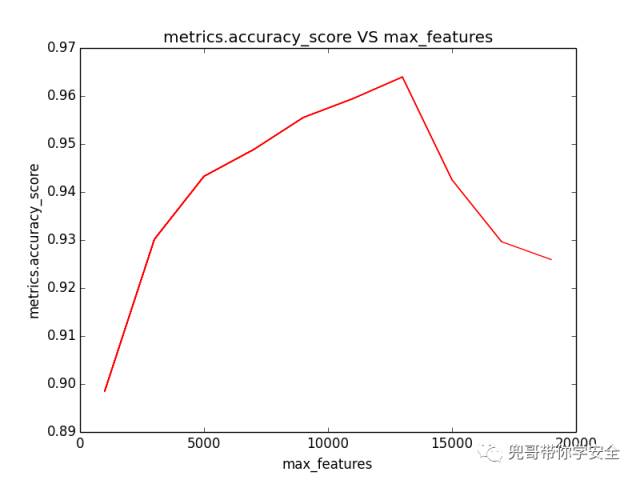
词袋最大特征树对朴素贝叶斯算法预测结果的影响
当max_features设置为13000时系统运行结果为:
CountVectorizer(analyzer=u'word', binary=False, decode_error='ignore',
dtype=<type 'numpy.int64'>, encoding=u'utf-8', input=u'content',
lowercase=True, max_df=1.0, max_features=13000, min_df=1,
ngram_range=(1, 1), preprocessor=None, stop_words='english',
strip_accents='ascii', token_pattern=u'(?u)\\b\\w\\w+\\b',
tokenizer=None, vocabulary=None)
0.963965299918
[[6369 200]
[ 286 6632]]
使用朴素贝叶斯算法,特征提取使用TF-IDF模型,将数据集合随机分配成训练集合和测试集合,其中测试集合比例为40%。
x_train, x_test, y_train, y_test = train_test_split(x, y, test_size = 0.4, random_state = 0)
gnb = GaussianNB()
gnb.fit(x_train,y_train)
y_pred=gnb.predict(x_test)
评估结果的准确度和TT、FF、TF、FT四个值。
print metrics.accuracy_score(y_test, y_pred)
print metrics.confusion_matrix(y_test, y_pred)
在词袋最大特征数为5000的情况下,整个系统准确度为95.91%,TT、FF、TF、FT矩阵如表所示,同等条件下准确率比词袋模型提升。
表1-2 基于TF-IDF模型的朴素贝叶斯验证结果
| 类型名称 | T | F |
| T | 6471 | 98 |
| F | 453 | 6465 |
完整输出结果为:
CountVectorizer(analyzer=u'word', binary=True, decode_error='ignore',
dtype=<type 'numpy.int64'>, encoding=u'utf-8', input=u'content',
lowercase=True, max_df=1.0, max_features=5000, min_df=1,
ngram_range=(1, 1), preprocessor=None, stop_words='english',
strip_accents='ascii', token_pattern=u'(?u)\\b\\w\\w+\\b',
tokenizer=None, vocabulary=None)
TfidfTransformer(norm=u'l2', smooth_idf=False, sublinear_tf=False,
use_idf=True)
NB and wordbag
0.959145844146
[[6471 98]
[ 453 6465]]
方法二:支持向量基算法
使用支持向量基算法,特征提取使用词袋模型,将数据集合随机分配成训练集合和测试集合,其中测试集合比例为40%。
x_train, x_test, y_train, y_test = train_test_split(x, y, test_size = 0.4, random_state = 0)
clf = svm.SVC()
clf.fit(x_train, y_train)
y_pred = clf.predict(x_test)
评估结果的准确度和TT、FF、TF、FT四个值。
print metrics.accuracy_score(y_test, y_pred)
print metrics.confusion_matrix(y_test, y_pred)
在词袋最大特征数为5000的情况下,整个系统准确度为90.61%,TT、FF、TF、FT矩阵如表1-3 所示,同等条件下准确率比词袋模型提升。
表1-3 基于词袋模型的SVM验证结果
| 类型名称 | T | F |
| T | 5330 | 1239 |
| F | 27 | 6891 |
完整输出结果为:
CountVectorizer(analyzer=u'word', binary=False, decode_error='ignore',
dtype=<type 'numpy.int64'>, encoding=u'utf-8', input=u'content',
lowercase=True, max_df=1.0, max_features=5000, min_df=1,
ngram_range=(1, 1), preprocessor=None, stop_words='english',
strip_accents='ascii', token_pattern=u'(?u)\\b\\w\\w+\\b',
tokenizer=None, vocabulary=None)
SVM and wordbag
0.906131830652
[[5330 1239]
[ 27 6891]]
1.1.3 方法三:深度学习算法之MLP
近几年有学者尝试使用深度学习算法提高垃圾邮件识别率。
我们先使用深度学习算法最简单的一种MLP(Multi-layer Perceptron,多层感知机),我们构造包括两层隐藏层的MLP,每层节点数分别为5和2,结构如图所示。
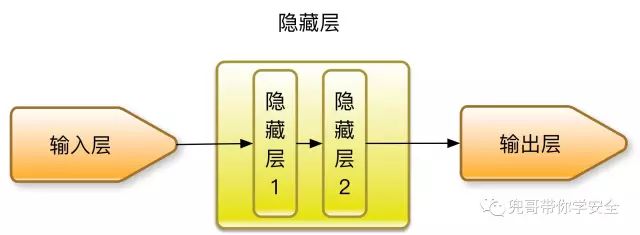
用于垃圾邮件检测的MLP结构图
在Scikit-Learn中可以使用MLPClassifier实现MLP,使用支持向量基算法,特征提取使用词袋模型,将数据集合随机分配成训练集合和测试集合,其中测试集合比例为40%。
x_train, x_test, y_train, y_test = train_test_split(x, y, test_size = 0.4, random_state = 0)
clf = MLPClassifier(solver='lbfgs',
alpha=1e-5,
hidden_layer_sizes = (5, 2),
random_state = 1)
clf.fit(x_train, y_train)
y_pred = clf.predict(x_test)
评估结果的准确度和TT、FF、TF、FT四个值。
print metrics.accuracy_score(y_test, y_pred)
print metrics.confusion_matrix(y_test, y_pred)
在词袋最大特征数为5000的情况下,整个系统准确度为98.01%,TT、FF、TF、FT矩阵如表1-4 所示,同等条件下准确率比词袋模型提升。
表1-4 基于词袋模型的MLP验证结果
| 类型名称 | T | F |
| T | 6406 | 163 |
| F | 105 | 6813 |
完整输出结果为:
DNN and wordbag
maxlen=5000
MLPClassifier(activation='relu', alpha=1e-05, batch_size='auto', beta_1=0.9,
beta_2=0.999, early_stopping=False, epsilon=1e-08,
hidden_layer_sizes=(20, 5, 2), learning_rate='constant',
learning_rate_init=0.001, max_iter=200, momentum=0.9,
nesterovs_momentum=True, power_t=0.5, random_state=1, shuffle=True,
solver='lbfgs', tol=0.0001, validation_fraction=0.1, verbose=False,
warm_start=False)
0.980129013124
[[6406 163]
[ 105 6813]]
1.1.4 方法四:深度学习算法之CNN
CNN的诞生是为了解决图像处理领域计算量巨大而无法进行深度学习的问题,CNN通过卷积计算、池化等大大降低了计算量,同时识别效果还满足需求。图像通常是二维数组,文字通常都是一维数据,是否可以通过某种转换后,也使用CNN对文字进行处理呢?答案是肯定的。
我们回顾下在图像处理时,CNN是如何处理二维数据的。如图所示,CNN使用二维卷积函数处理小块图像,提炼高级特征进一步分析。典型的二维卷积函数处理图片的大小为3*3、4*4等。

CNN处理图像数据的过程
同样的原理,我们可以使用一维的卷积函数处理文字片段,提炼高级特征进一步分析。典型的一维卷积函数处理文字片段的大小为3、4、5等。
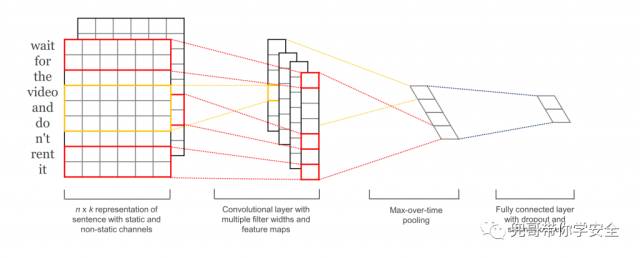
CNN处理文本数据的过程
这个要感谢Yoon Kim的经典论文Convolutional Neural Networks for Sentence Classification
言归正传,使用词汇表编码后,将数据集合随机分配成训练集合和测试集合,其中测试集合比例为40%。
x,y=get_features_by_tf()
x_train, x_test, y_train, y_test = train_test_split(x, y, test_size = 0.4, random_state = 0)
将训练和测试数据进行填充和转换,不到最大长度的数据填充0,由于是二分类问题,把标记数据二值化。定义输入参数的最大长度为文档的最大长度。
trainX = pad_sequences(trainX, maxlen=max_document_length, value=0.)
testX = pad_sequences(testX, maxlen=max_document_length, value=0.)
# Converting labels to binary vectors
trainY = to_categorical(trainY, nb_classes=2)
testY = to_categorical(testY, nb_classes=2)
network = input_data(shape=[None,max_document_length], name='input')
定义CNN模型,其实使用3个数量为128核,长度分别为3、4、5的一维卷积函数处理数据。
network = tflearn.embedding(network, input_dim=1000000, output_dim=128)
branch1 = conv_1d(network, 128, 3, padding='valid', activation='relu', regularizer="L2")
branch2 = conv_1d(network, 128, 4, padding='valid', activation='relu', regularizer="L2")
branch3 = conv_1d(network, 128, 5, padding='valid', activation='relu', regularizer="L2")
network = merge([branch1, branch2, branch3], mode='concat', axis=1)
network = tf.expand_dims(network, 2)
network = global_max_pool(network)
network = dropout(network, 0.8)
network = fully_connected(network, 2, activation='softmax')
network = regression(network, optimizer='adam', learning_rate=0.001,
loss='categorical_crossentropy', name='target')
实例化CNN对象并进行训练数据,一共训练5轮。
model = tflearn.DNN(network, tensorboard_verbose=0)
model.fit(trainX, trainY,
n_epoch=5, shuffle=True, validation_set=(testX, testY),
show_metric=True, batch_size=100,run_id="spam")
CNN的结构如图所示。
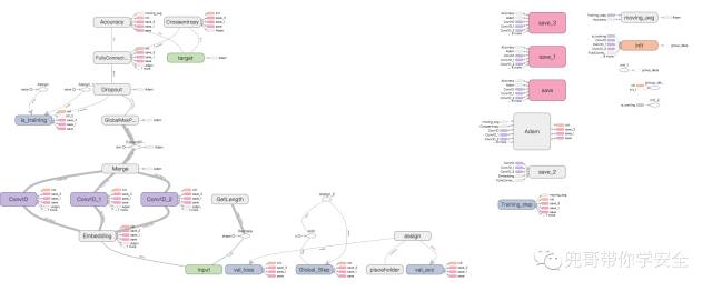
处理垃圾邮件的CNN结构图
在我的mac本上运行了近3个小时后,对测试数据集的识别准确度达到了令人满意的98.30%。
Training Step: 680 | total loss: 0.01691 | time: 2357.838s
| Adam | epoch: 005 | loss: 0.01691 - acc: 0.9992 | val_loss: 0.05177 - val_acc: 0.9830 -- iter: 13524/13524
--
1.1.5 方法五:深度学习算法之RNN
RNN由于特殊的结构,可以使用以前的记忆协助分析当前的数据,这点非常适合语言文本相关任务的处理,因此在NLP等领域使用广泛。
我们使用词汇表编码后,将数据集合随机分配成训练集合和测试集合,其中测试集合比例为40%。
x,y=get_features_by_tf()
x_train, x_test, y_train, y_test = train_test_split(x, y, test_size = 0.4, random_state = 0)
将训练和测试数据进行填充和转换,不到最大长度的数据填充0,由于是二分类问题,把标记数据二值化。定义输入参数的最大长度为文档的最大长度。
trainX = pad_sequences(trainX, maxlen=max_document_length, value=0.)
testX = pad_sequences(testX, maxlen=max_document_length, value=0.)
# Converting labels to binary vectors
trainY = to_categorical(trainY, nb_classes=2)
testY = to_categorical(testY, nb_classes=2)
network = input_data(shape=[None,max_document_length], name='input')
定义RNN结构,使用最简单的单层LSTM结构。
# Network building
net = tflearn.input_data([None, max_document_length])
net = tflearn.embedding(net, input_dim=1024000, output_dim=128)
net = tflearn.lstm(net, 128, dropout=0.8)
net = tflearn.fully_connected(net, 2, activation='softmax')
net = tflearn.regression(net, optimizer='adam', learning_rate=0.001,
loss='categorical_crossentropy')
实例化RNN对象并进行训练数据,一共训练5轮。
# Training
model = tflearn.DNN(net, tensorboard_verbose=0)
model.fit(trainX, trainY, validation_set=(testX, testY), show_metric=True,
batch_size=10,run_id="spm-run",n_epoch=5)
RNN的结构如图所示。
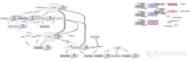
处理垃圾邮件的RNN结构图
在我的mac本上运行了近3个小时后,对测试数据集的识别准确度达到了尚可的94.88%。
小结
本文以Enron-Spam数据集为训练和测试数据集,介绍了常见的垃圾邮件识别方法,介绍了三种特征提取方式,分别是词袋模型、TF-IDF模型和词汇表模型,其中词汇表模型后来发展成了word2ver模型,这个会在后面章节具体介绍。
本章介绍了常见的垃圾邮件分类算法,包括朴素贝叶斯、支持向量机以及深度学习的三种算法,其中CNN和MLP算法的识别率达到了令人满意的98%以上。
值得一提的是,在朴素贝叶斯的实验中我们发现,词袋抽取的单词个数并非越多,垃圾邮件识别概率越大,而是有个中间点可以达到效果最佳,并且TF-IDF结合词袋模型会提升检测能力,后面章节我们都会结合两者使用。
以上提到的各种方法基本都有大量参数可以调优,比如神经网络的层数,取样的文本长度等,由于篇幅有限不一一赘述。
另外,针对英文环境,在特征提取环节还有调优空间,比如动词的不同时态、名词的单复数的归一化处理,常用的停顿词诸如the的处理等。
1.2.1 参考文献
l https://wenku.baidu.com/view/e41634fdcc22bcd127ff0c6b.html
l http://scikit-learn.org/stable/modules/generated/sklearn.feature_extraction.text.CountVectorizer.html#sklearn.feature_extraction.text.CountVectorizer
l http://www2.aueb.gr/users/ion/data/enron-spam/
l http://blog.csdn.net/u013713117/article/details/69261769
l C.D. Manning, P. Raghavan and H. Schütze (2008). Introduction to Information Retrieval. Cambridge University Press, pp. 234-265.
l McCallum and K. Nigam (1998). A comparison of event models for Naive Bayes text classification. Proc. AAAI/ICML-98 Workshop on Learning for Text Categorization, pp. 41-48.
l V. Metsis, I. Androutsopoulos and G. Paliouras (2006). Spam filtering with Naive Bayes – Which Naive Bayes? 3rd Conf. on Email and Anti-Spam (CEAS).
l http://news.ifeng.com/a/20140725/41314715_0.shtml?f=hao123
l http://scikit-learn.org/stable/modules/svm.html#svm
l Ali Rodan, Hossam Faris, Ja’far Alqatawna,Optimizing Feedforward Neural Networks Using Biogeography Based Optimization for E-Mail Spam Identification,Int. J. Communications, Network and System Sciences, 2016, 9, 19-28
l Guzella, T.S. and Caminhas, W.M. (2009) A Review of Machine Learning Approaches to Spam Filtering. Expert Sys- tems with Applications, 36, 10206-10222.
l http://dx.doi.org/10.1016/j.eswa.2009.02.037
l Rao, J.M. and Reiley, D.H. (2012) The Economics of Spam. The Journal of Economic Perspectives, 26, 87-110. http://dx.doi.org/10.1257/jep.26.3.87
l Stern, H., et al. (2008) A Survey of Modern Spam Tools. CiteSeer.
l Su, M.-C., Lo, H.-H. and Hsu, F.-H. (2010) A Neural Tree and Its Application to Spam E-Mail Detection. Expert Sys- tems with Applications, 37, 7976-7985.
l http://dx.doi.org/10.1016/j.eswa.2010.04.038
l Kanich, C., Weaver, N., McCoy, D. Halvorson, T., Kreibich, C., Levchenko, K., Paxson, V., Voelker, G.M. and Sa- vage, S. (2011) Show Me the Money: Characterizing Spam-Advertised Revenue. USENIX Security Symposium, 15.
l http://www.chinaz.com/web/2012/0521/252930.shtml
l http://scikit-learn.org/stable/modules/feature_extraction.html#tfidf-term-weighting
l http://scikit-learn.org/dev/modules/neural_networks_supervised.html#multi-layer-perceptron
l “Learning representations by back-propagating errors.” Rumelhart, David E., Geoffrey E. Hinton, and Ronald J. Williams.
l “Stochastic Gradient Descent” L. Bottou - Website, 2010.
l “Backpropagation” Andrew Ng, Jiquan Ngiam, Chuan Yu Foo, Yifan Mai, Caroline Suen - Website, 2011.
l “Efficient BackProp” Y. LeCun, L. Bottou, G. Orr, K. Müller - In Neural Networks: Tricks of the Trade 1998.
l “Adam: A method for stochastic optimization.” Kingma, Diederik, and Jimmy Ba. arXiv preprint arXiv:1412.6980 (2014)
l Andrew L. Maas, Raymond E. Daly, Peter T. Pham, Dan Huang, Andrew Y. Ng,and Christopher Potts. (2011).Learning Word Vectors for Sentiment Analysis. The 49th Annual Meeting of the Association for Computational Linguistics (ACL 2011)
l http://www.wildml.com/2015/12/implementing-a-cnn-for-text-classification-in-tensorflow/
l Yoon Kim,Convolutional Neural Networks for Sentence Classification,EMNLP 2014
l http://www.wildml.com/2015/11/understanding-convolutional-neural-networks-for-nlp/
l https://github.com/clayandgithub/zh_cnn_text_classify
本文来自兜哥带你学安全,原文链接:兜哥带你学安全
文章图片来源于网络,如有问题请联系我们